SUMPRODUCT (Returns the sum of the products of corresponding array components)

What Does It Do?

This function uses at least two columns of values.

The values in the first column are multipled with the corresponding value in the second column.

The total of all the values is the result of the calculation.

Syntax

=SUMPRODUCT(Range1, Range, Range3 through to Range30)

Formatting

No special formatting is required.

Example

The following table was used by a drinks merchant to keep track of stock.

The merchant needed to know the total purchase value of the stock, and the potential value of the stock when it is sold, takinging into account the markup percentage.

The =SUMPRODUCT() function is used to multiply the Cases In Stock with the Case Price to calculate what the merchant spent in buying the stock.

The =SUMPRODUCT() function is used to multiply the Cases In Stock with the Bottles In Case and the Bottle Setting Price, to calculate the potential value of the stock if it is all sold.

SYD (Returns the sum-of-years' digits depreciation of an asset for a specified period)

What Does It Do?

This function calculates the depreciation of an item throughout its life, using the sum of the years digits.

The depreciation is greatest in the earlier part of the  items life.

What is the Sum Of The Years Digits ?

The sum of the years digits adds together the each of the years of the life.

A life of 3 years has a sum of 1+2+3 equalling 6.

Each of the years is then calculated as a percentage of the sum of the years.

Year 3 is 50% of 6, year 2 is 33% of 6, year 1 is 17% 6.

The total depreciation of the item is then allocated on the basis of these percentages.

A depreciation of Rs. 9000 is allocated as 50% being Rs. 4500, 33% being Rs. 3000, 17% being Rs. 1500.

As the greater part of the depreciation is allocated to the earliest years the values are inverted, year 1 is Rs. 4500, year 2 is Rs. 3000 and year 1 is Rs. 1500.

Example-1

1. Add together the digits of the Life to get the SumOfTheYearsDigits, 1+2+3=6.

2. Subtract the Salvage from the Purchase Price to get Total Deprectation, 10000-1000= 9000.

3. Divide the Total Deprectation by the SumOfTheYearsDigits, 9000/6=1500.

4. Invert the year digits, 1,2,3 becomes 3,2,1.

5. Multiply 3,2,1 by £1500 to get 4500, 3000,1500, these values are the depreciation    values for each of the three years in the life of the item.

Example-2

The same example using 4 years.

Example-3

This is example will adjust itself to accommodate any number of years between 1 and 10.

Syntax

=SYD(OriginalCost,SalvageValue,Life,PeriodToCalculate)

Formatting

No special formatting is required.

T (Converts its arguments to text)

What Does It Do?

This function examines an entry to determine whether it is text or not.

If the value is text, then the text is the result of the function

If the value is not text, the result is a blank.

The function is not specifically needed by Excel, but is included for compatibility with other spreadsheet programs.

Syntax

=T(CellToTest)

Formatting

No special formatting is required.

TEXT (Formats a number and converts it to text)

What Does It Do?

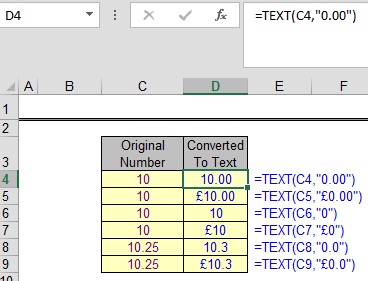
This function converts a number to a piece of text.

The formatting for the text needs to be specified in the function.

Syntax

=TEXT(NumberToConvert,FormatForConversion)

Formatting

No special formatting is required.