ISERR (Returns TRUE if the value is any error value except #N/A)

What Does It Do?

This function tests a cell and shows TRUE if there is an error value in the cell.

It will show FALSE if the contents of the cell calculate without an error, or if the error is the #NA message.

Syntax

=ISERR(CellToTest)

The CellToTest can be a cell reference or a calculation.

Formatting

No special formatting is needed.

Example

The following tables were used by a publican to calculate the cost of a single bottle of champagne, by dividing the cost of the crate by the quantity of bottles in the crate.

Table 1 shows what happens when the value zero 0 is entered as the number of bottles.

The #DIV/0 indicates that an attempt was made to divide by zero 0, which Excel does not do.

Table 2 shows how this error can be trapped by using the =ISERR() function.

ISERROR (Returns TRUE if the value is any error value)

What Does It Do?

This function tests a cell or calculation to determine whether an error has been generated.

It will show TRUE for any type of error and FALSE if no error is found.

Syntax

=ISERROR(CellToTest)

The CellToTest can be a cell reference or a formula.

Formatting

No special formatting is needed.

Example

The following tables was used to calculate the difference between two dates.

Table 1 shows an error due to the fact that the first entry was entered using an inappropriate date format.

Table 2 shows how the =ISERROR() function has been used to trap the error and inform the user that there has been an error in the data entry.

ISEVEN (Returns TRUE if the number is even)

What Does It Do?

This function tests a number to determine whether it is even.

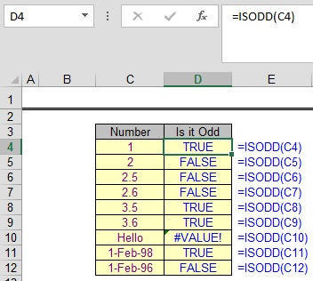
An even number is shown as TRUE an odd number is shown as FALSE.

Note that decimal fractions are ignored.

Note that dates can be even or odd.

Note that text entries result in the #VALUE! error.

Syntax

=ISEVEN(CellToTest)

Formatting

No special formatting is needed.

ISLOGICAL (Returns TRUE if the value is a logical value)

What Does It Do?

This function tests a cell to determine whether the cell contents are logical.

The logical values can only be TRUE or FALSE.

If the cell does contain a logical value, the result TRUE is shown.

If the cell does not contain a logical value, the result FALSE is shown.

Syntax

=ISLOGICAL(CellToTest)

Formatting

No special formatting is needed.

ISNA (Returns TRUE if the value is the #N/A error value)

What Does It Do?

This function tests a cell to determine whether it contains the Not Available error #N/A.

The #N/A is generated when a function cannot work properly because of missing data.

The #N/A can also be typed in to a cell by the user to indicate the cell is currently empty, but will be used for data entry in the future.

The function is normally used with other functions such as the =IF() function.

Syntax

=ISNA(CellToTest)

Formatting

No special formatting is needed.

ISNONTEXT (Returns TRUE if the value is not text)

What Does It Do?

This functions tests an entry to determine whether it is a number, rather than text.

It would be used to ensure that only numeric entries are used in calculations, rather than text which looks like a number, such as typing the letter O instead of zero 0.

The function is normally used with other function such as the =IF() function.

Syntax

=ISNONTEXT(CellToTest)

Formatting

No special formatting is needed.

Example

The following table is used by an electrical retailer to calculate the selling price of an item based on the buying price and the shop mark-up.

Table 1 shows the #VALUE! error generated when a number, 300, is entered using the letter O instead of the zero 0.

Table 2 shows how the error is trapped using the =ISNONTEXT function and the =IF() function in the calculation.

ISNUMBER (Returns TRUE if the value is a number)

What Does It Do?

This function examines a cell or calculation to determine whether it is a numeric value.

If the cell or calculation is a numeric value the result TRUE is shown.

If the cell or calculation is not numeric, or is blank, the result FALSE is shown.

Syntax

=ISNUMBER(CellToTest)

The cell to test can be a cell reference or a calculation.

Formatting

No special formatting is needed.

Example

The following table was used by a personnel department to lookup the salary of an employee.

The employee can be entered as a Name or as a Numeric value.

The =ISNUMBER() function has been used to identify the type of entry made, and then

the =IF() decides which VLOOKUP to perform.

ISODD (Returns TRUE if the number is odd)

What Does It Do?

This function tests a number to determine whether it is odd.

An odd number is shown as TRUE an even number is shown as FALSE.

Note that decimal fractions are ignored.

Note that dates can be odd or even.

Note that text entries result in the #VALUE! error.

Syntax

=ISODD(CellToTest)

Formatting

No special formatting is needed.

ISREF (Returns TRUE if the value is a reference)

What Does It Do?

This function shows TRUE if given a cell address, or FALSE for any other type of value.

Its a bit of an odd one, and is normally used in macros rather than on the worksheet.

Syntax

=ISREF(ValueToTest)

The ValueToTest can be any type of data, but when used on the worksheet, it cannot be a reference to the contents of another cell, as the reference will itself be evaluated by the function.

Formatting

No special formatting is needed.

ISTEXT (Returns TRUE if the value is text)

What Does It Do?

This functions tests an entry to determine whether it is text.

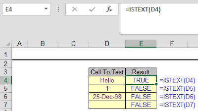
If the entry is text is shows TRUE.

If the entry is any other type it shows FALSE.

Syntax

=ISTEXT(CellToTest)

Formatting

No special formatting is needed.

Example

The following table was used by a personnel department to lookup the salary of an employee.

The employee can be entered as a Name or as a Numeric value.

The =ISTEXT() function has been used to identify the type of entry made, and then the =IF() decides which VLOOKUP to perform.

LARGE (Returns the k-th largest value in a data set)

What Does It Do?

This function examines a list of values and picks the value at a user specified position in the list.

Syntax

=LARGE(ListOfNumbersToExamine,PositionToPickFrom)

Formatting

No special formatting is needed.

Example

The following table was used to calculate the top 3 sales figures between Jan, Feb and Mar.

Note

Another way to find the Highest and Lowest values would have been to use the =MAX() and =MIN() functions.

LCM (Returns the least common multiple)

What Does It Do?

This function calculate the Least Common Multiple, which is the smallest number that can be divided by each of the given numbers.

Syntax

=LCM(Number1,Number2,Number3... through to Number29)

Formatting

No special formatting is needed.

LEFT (Returns the leftmost characters from a text value)

What Does It Do?

This function displays a specified number of characters from the left hand side of a piece of text.

Syntax

=LEFT(OriginalText,NumberOfCharactersRequired)

Formatting

No special formatting is needed.

Example

The following table was used to extract the first name of a person from their full name.

The =FIND() function was used to locate position of the space between the first and second name.

The length of the first name is therefore the position of the space minus one character.

The =LEFT() function can now extract the first name based on the position of the space.

LEN (Returns the number of characters in a text string)

What Does It Do?

This function counts the number of characters, including spaces and numbers, in a piece of text.

Syntax

=LEN(Text)

Formatting

No special formatting is needed.

Example

This example shows how the =LEN() function is used in a formula which extracts the second name from a text entry containing both first and second names.

LOOKUP - Array

What Does It Do?

This function looks for a piece of information in a list, and then picks an item from the last cell in the adjacent row or column.

It always picks the data from the end of the row or column, so it is no good if you need to pick data from part way across a list, (use VLOOKUP or HLOOKUP).

The way in which the function decides whether to pick from the row or column is based on the size of the table.

Syntax

=LOOKUP(WhatToLookFor,RangeToLookIn)

The WhatToLookFor should be a single item.

The RangeToLook in can be either horizontal or vertical.

Be careful not to include unnecessary heading in the range as these will cause errors.

Formatting

No special formatting is needed.

Problem

The list of information to be looked through must be sorted in ascending order, otherwise errors will occur, either as #N/A or incorrect results.

Table 1 shows the Name column sorted alphabetically, the results of using =LOOKUP() will be correct.

Table 2 shows the same data, but not sorted. Sometimes the results will be correct, but other times the result will be an #N/A error or incorrect figure.