Roundup (Rounds a number up, away from zero)

What Does It Do?

This function rounds a number up to a specified amount of decimal places.

If 0 is used the number is rounded up to the nearest whole number.

If a negative amount of rounding is used the figures to the left of the decimal point are rounded.

Syntax

=ROUNDUPNumberToRound,DecimalPlacesToUse)

Formatting

No special formatting is needed.

Second (Converts a serial number to a second)

What Does It Do?

The function will show the second of the minute based upon a time or a number.

Only the fraction part of the number is used as it is this which relates to time of day.

Syntax

=SECOND(Number)

Formatting

The result will be shown as a normal number between 0 and 59.

Example

The following table was used by a telephone compnay to calculate the cost of a call.

The telephone company only deals in seconds which are a multiple of 5.

The seconds in a call are rounded up to the nearest multiple of 5 before the bill is calculated.

The Duration of the call is entered.

The =MINUTES() function calculates the total number of minutes.

The =SECOND() function calculates the total number of seconds.

The =CEILING() function rounds the seconds up to the nearest muliple of 5.

The Cost of the call is then calculated.

Sign (Returns the sign of a number for Mathematical Purpose)

What Does It Do?

This function tests a value to determine whether it is positive or negative.

If the value is positive the result is 1.

If the value is negative the result is -1.

If the value is zero 0 the result is 0.

Syntax

=SIGN(CellToTest)

The CellToTest can be a cell or a calculation.

Formatting

No special formatting is needed.

SLN (Returns the straight-line depreciation of an asset for one period for Financial Purpose)

What Does It Do?

This function calculates the Straight Line Depreciation of an item.

(Also known as Fixed Instalment method).

The Straight Line Depreciation is how much the value of an item reduced during a specific period of time. The result is a uniform depreciation value.

An example would be if you bought a new car for Rs. 20,000, then kept it for 6 years.

At the end of your ownership you sell the car for Rs. 8,000.

The difference between the original and the trade in price is Rs. 20,000 - Rs. 8,000 which is Rs. 12,000.

Because you owned the car for 6 years, the SLN is calculated as Rs. 12,000 / 6 which is Rs. 2,000.

Syntax

=SLN(OriginalCost,SellingPrice,LengthOfOwnership)

The LengthOfOwnership can be any time period, days, months or years.

However, the SLN which is calculated will, be for that time, specifying 2 years ownership as 24 months will give an SLN per month.

Formatting

No special formatting is needed.

Small (Returns the k-th smallest value in a data set for Statistical Purpose)

What Does It Do?

This function examines a list of values and picks the value at a user specified position in the list.

Syntax

=SMALL(ListOfNumbersToExamine,PositionToPickFrom)

Formatting

No special formatting is needed.

Example

The following table was used to calculate the bottom 3 sales figures between Jan, Feb and Mar.

Note

Another way to find the Highest and Lowest values would have been to use the =MAX() and =MIN() functions.

STDEV (Estimates standard deviation based on a sample)

What Does It Do?

This function calculates the sample population standard deviation of a list of values.

A sample population is used when the list of values represents a sample of a population.

Syntax

=STDEV(Range1,Range2,Range3 through to Range30)

Formatting

No special formatting is needed.

Example

The table below was used by a company interested in buying a new machine to pack washing powder.

Three machines were short listed and allow to run for a day.

At the end of the day four boxes of soap powder were picked at random from the production of each machine.

The boxes were weighed and the =STDEV() function used as these boxes only represented a sample of the complete days production.

The machine with the smallest deviation was the most consistent.

Explanation of Formula:

This finds the lowest value:                                =MIN(H34:H36)

This finds the position of the lowest value:         =MATCH(MIN(H34:H36),H34:H36,0)

This looks down the Machine column to

find the machine name:                         =INDEX(C34:C36,MATCH(MIN(H34:H36),H34:H36,0))

STDEVP (Calculates standard deviation based on the entire population)

What Does It Do?

This function calculates the standard deviation of a list of values.

The result is calculated on the basis that the values represent the entire population.

Syntax

=STDEVP(Range1,Range2,Range3 through to Range30)

Formatting

No special formatting is needed.

Example

The table below was used by a company interested in buying a new machine to pack washing powder.

A trial run of just four boxes per machine were produced.

The boxes were weighed and the =STDEVP() function used as these boxes represented the entire test run.

The machine with the smallest variance was the most consistent. ????????????????????

Explanation of formula:

·         This finds the lowest value:                                =(MIN(H32:H34)

·         This finds the position of the lowest value.:        =MATCH(MIN(H32:H34),H32:H34,0)

·         This looks down the Machine column to

find the machine name:  =INDEX(C32:C34,MATCH(MIN(H32:H34),H32:H34,0))

SUBSTITUTE (Substitutes new text for old text in a text string)

This function replaces a specified piece of text with a different piece of text.

It can either replace all occurrences of the text, or a specific instance.

The function is case sensitive.

Syntax

=SUBSTITUTE(OriginalText,TextToRemove,TextToInsert,InstanceToUse)

The InstanceToUse is optional, if it is omitted all instances will be substituted.

Formatting

No special formatting is needed.

Note

To cope with upper or lower case in the substitution you can use other text functions such as =UPPER(), =LOWER() or =PROPER() to ensure that the substitution will take place.

Table 1 shows how differing text cases alter the result of the substitution.

Table 2 shows how the =PROPER() function has been used to take account of the mixed cases.

SUM (Adds its arguments)

What Does It Do ?

This function creates a total from a list of numbers.

It can be used either horizontally or vertically.

The numbers can be in single cells, ranges are from other functions.

Syntax

=SUM(Range1,Range2,Range3... through to Range30).

Formatting

No special formatting is needed.

Note

Many people use the =SUM() function incorrectly.

This example shows how the SUM has been combined with plus + symbols.

The formula is actually doing more work than needed.

It should have been entered as either =C48+C49+C50 or =SUM(C48:C50).

SUM-Running Total (Using in Sampling)

Using =SUM() For A Running Total

Type the formula =SUM($D$7:D7) in cell E7 and then copy down the table. It works because the first reference uses dollar symbols $ to keep $D$7 static as the formula is copied down. Each occurrence of the =SUM() then adds all the numbers from the first cell down.

The function can be tidied up to show 0 zero when there is no adjacent value by using the =IF() function.

SUM and the =OFFSET function (Sample)

Sometimes it is necessary to base a calculation on a set of cells in different locations.

An example would be when a total is required from certain months of the year, such as the last 3 months in relation to the current date.

One solution would be to retype the calculation each time new data is entered, but this would be time consuming and open to human error.

A better way is to indicate the start and end point of the range to be calculated by using the =OFFSET() function.

The =OFFSET() picks out a cell a certain number of cells away from another cell. By giving the =OFFSET() the address of the first cell in the range which needs to be totalled, we can then indicate how far away the end cell should be and the =OFFSET()will give us the address of cell which will be the end of the range to be totalled.

The =OFFSET() needs to know three things;

1. A cell address to use as the fixed point from where it should base the offset.

2. How many rows it should look up or down from the starting point.

3. How many columns it should look left or right from the starting point.

Using =OFFSET() Twice In A Formula

The following examples use =OFFSET() to pick both the start and end of the range which needs to be totalled.

Example

The following table shows five months of data.

To calculate the total of a specific group of months the =OFFSET() function has been used.

 The Start and End dates entered in cells F71 and F72 are used as the offset to produce a range which can be totalled.

Explanation

The following formula represent a breakdown of what the =OFFSET function does.

The  formula displayed below are only dummies, but they will update as you enter dates into cells F71 and F72.

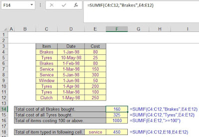
SUMIF (Adds the cells specified by a given criteria)

What Does It Do?

This function adds the value of items which match criteria set by the user.

Syntax

=SUMIF(RangeOfThingsToBeExamined,CriteriaToBeMatched,RangeOfValuesToTotal)

=SUMIF(C4:C12,"Brakes",E4:E12)                      This examines the names of products in C4:C12.

                                                                        It then identifies the entries for Brakes.

                                                                        It then totals the respective figures in E4:E12

=SUMIF(E4:E12,">=100")                                   This examines the values in E4:E12.

                                                                        If the value is >=100 the value is added to the total.

Formatting

No special formatting is required.